System Reliability and Availability
We have already discussed reliability and availability basics in a previous article. This article will focus on techniques for calculating system availability from the availability information for its components.
The following topics are discussed in detail:
System Availability
System Availability is calculated by modeling the system as an interconnection of parts in series and parallel. The following rules are used to decide if components should be placed in series or parallel:
- If failure of a part leads to the combination becoming inoperable, the two parts are considered to be operating in series
- If failure of a part leads to the other part taking over the operations of the failed part, the two parts are considered to be operating in parallel.
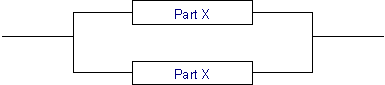
Availability in Series

As stated above, two parts X and Y are considered to be operating in series if failure of either of the parts results in failure of the combination. The combined system is operational only if both Part X and Part Y are available. From this it follows that the combined availability is a product of the availability of the two parts. The combined availability is shown by the equation below:
A = Ax Ay
The implications of the above equation are that the combined availability of two components in series is always lower than the availability of its individual components. Consider the system in the figure above. Part X and Y are connected in series. The table below shows the availability and downtime for individual components and the series combination.
| Component | Availability | Downtime |
| X | 99% (2-nines) | 3.65 days/year |
| Y | 99.99% (4-nines) | 52 minutes/year |
| X and Y Combined | 98.99% | 3.69 days/year |
From the above table it is clear that even though a very high availability Part Y was used, the overall availability of the system was pulled down by the low availability of Part X. This just proves the saying that a chain is as strong as the weakest link. More specifically, a chain is weaker than the weakest link.
Availability in Parallel
As stated above, two parts are considered to be operating in parallel if the combination is considered failed when both parts fail. The combined system is operational if either is available. From this it follows that the combined availability is 1 - (both parts are unavailable). The combined availability is shown by the equation below:
A = 1-(1-Ax )2
The implications of the above equation are that the combined availability of two components in parallel is always much higher than the availability of its individual components. Consider the system in the figure above. Two instances of Part X are connected in parallel. The table below shows the availability and downtime for individual components and the parallel combination.
| Component | Availability | Downtime |
| X | 99% (2-nines) | 3.65 days/year |
| Two X components operating in parallel | 99.99% (4-nines) | 52 minutes/year |
| Three X components operating in parallel | 99.9999% (6-nines) | 31 seconds /year ! |
From the above table it is clear that even though a very low availability Part X was used, the overall availability of the system is much higher. Thus parallel operation provides a very powerful mechanism for making a highly reliable system from low reliability. For this reason, all mission critical systems are designed with redundant components. (Different redundancy techniques are discussed in the Hardware Fault Tolerance article)
Partial Operation Availability
Consider a switching system. Call Processors handle the call processing for digital trunks. The system has been designed to incrementally add call processor cards to handle subscriber load. Now consider the case of a switch configured with 10 call processor cards. Should we consider the system to be unavailable when one call processor card fails? This doesn't seem right, as 90% of subscribers are still being served.
In such systems where failure of a component leads to some users losing service, system availability has to be defined by considering the percentage of users affected by the failure. For example, in a switching system the system might be considered unavailable if 30% of the subscribers are affected. This translates to 3 call processor cards out of 10 failing. We need a formula to calculate the availability when a system with 7 Switching cards is considered as available.
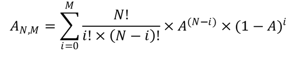
Consider a system with N components where the system is considered to be available when at least N-M components are available (i.e. no more than M components can fail). The availability of such a system is denoted by AN,M and is calculated below:
Availability Computation Example
In this section we will compute the availability of a simple signal processing system.
Understanding the System
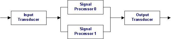
As a first step, we prepare a detailed block diagram of the system. This system consists of an input transducer which receives the signal and converts it to a data stream suitable for the signal processor. This output is fed to a redundant pair of signal processors. The active signal processor acts on the input, while the standby signal processor ignores the data from the input transducer. Standby just monitors the sanity of the active signal processor. The output from the two signal processor boards is combined and fed into the output transducer. Again, the active signal processor drives the data lines. The standby keeps the data lines tri-stated. The output transducer outputs the signal to the external world.
Input and output transducer are passive devices with no microprocessor control. The Signal processor cards run a real-time operating system and signal processing applications.
Also note that the system stays completely operational as long as at least one signal processor is in operation. Failure of an input or output transducer leads to complete system failure.
Reliability Modeling of the System
The second step is to prepare a reliability model of the system. At this stage we decide the parallel and serial connectivity of the system. The complete reliability model of our example system is shown below:
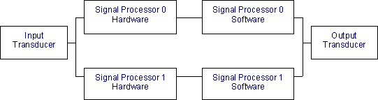
A few important points to note here are:
- The signal processor hardware and software have been modeled as two distinct entities. The software and the hardware are operating in series as the signal processor cannot function if the hardware or the software is not operational.
- The two signal processors (software + hardware) combine together to form the signal processing complex. Within the signal processing complex, the two signal processing complexes are placed in parallel as the system can function when one of the signal processors fails.
- The input transducer, the signal processing complex and the output transducer have been placed in series as failure of any of the three parts will lead to complete failure of the system.
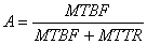
Calculating Availability of Individual Components
Third step involves computing the availability of individual components. MTBF (Mean time between failure) and MTTR (Mean time to repair) values are estimated for each component (See Reliability and Availability basics article for details). For hardware components, MTBF information can be obtained from hardware manufactures data sheets. If the hardware has been developed in house, the hardware group would provide MTBF information for the board. MTTR estimates for hardware are based on the degree to which the system will be monitored by operators. Here we estimate the hardware MTTR to be around 2 hours.
Once MTBF and MTTR are known, the availability of the component can be calculated using the following formula:
Estimating software MTBF is a tricky task. Software MTBF is really the time between subsequent reboots of the software. This interval may be estimated from the defect rate of the system. The estimate can also be based on previous experience with similar systems. Here we estimate the MTBF to be around 4000 hours. The MTTR is the time taken to reboot the failed processor. Our processor supports automatic reboot, so we estimate the software MTTR to be around 5 minute. Note that 5 minutes might seem to be on the higher side. But MTTR should include the following:
- Time wasted in activities aborted due to signal processor software crash
- Time taken to detect signal processor failure
- Time taken by the failed processor to reboot and come back in service
| Component | MTBF | MTTR | Availability | Downtime |
| Input Transducer | 100,000 hours | 2 hours | 99.998% | 10.51 minutes/year |
| Signal Processor Hardware | 10,000 hours | 2 hours | 99.98% | 1.75 hours/year |
| Signal Processor Software | 2190 hours | 5 minute | 99.9962% | 20 minutes/year |
| Output Transducer | 100,000 hours | 2 hours | 99.998% | 10.51 minutes/year |
Things to note from the above table are:
- Availability of software is higher, even though hardware MTBF is higher. The main reason is that software has a much lower MTTR. In other words, the software does fail often but it recovers quickly, thereby having less impact on system availability.
- The input and output transducers have fairly high availability, thus fairly high availability can be achieved even without redundant components.
Calculating System Availability
The last step involves computing the availability of the entire system. These calculations have been based on serial and parallel availability calculation formulas.
| Component | Availability | Downtime |
| Signal Processing Complex (software + hardware) | 99.9762% | 2.08 hours/year |
| Combined availability of Signal Processing Complex 0 and 1 operating in parallel | 99.99999% | 3.15 seconds/year |
| Complete System | 99.9960% | 21.08 minutes/year |